Introduction to Charts in MS Excel
In the next part of this training series I show you how to set up charts in Microsoft Excel.
Download this lesson on excel charts as a pdf: Introduction to Charts
To Create a chart using the Chart wizard
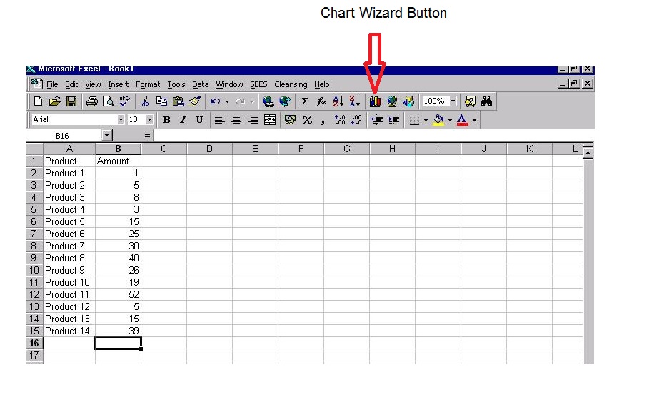
- Select the data on your worksheet, that you want to create the chart from.
- Click on the Chart Wizard button on the toolbar.
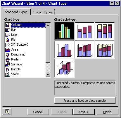
When you release the mouse button Step1 of the Chart Wizard will be displayed.
- Under the Chart type: option, click on the different chart types to view the types of chart that you want to create.
- Under the Chart sub type option, click on the sub-type you would like for your chart.
- To see how your data would look using a certain chart type, press and hold to view sample button.
- When you have found the type of chart you would like to create, click on the next button.
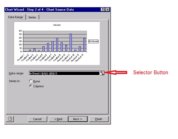
- Next to the data range option, check that the range you selected on your worksheet is correct, if the range is incorrect click on the selector button, reselect the range on your worksheet, and then click the selector button again.
Click the next button.
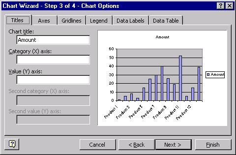
- Under the Chart title box, type in the title you would like for your chart, and any axis titles.
- Click on the Legend tab, and choose whether you would like a legend displayed, and its position.
- Click on the Data Labels tab, and choose whether you would like your data labelled.
- When you have finished choosing titles, legends, labels and any other details, click on the Next button.
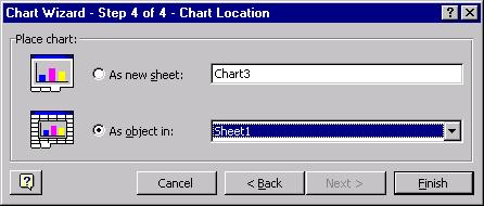
- The final part is to decide whether you would like your chart displayed as a new sheet or included on the same sheet as your data.
- Click on the Finish button.
Don’t forget you down download the introduction to charts as a PDF: Introduction to Charts
Other Lessons
- Introduction to Microsoft Excel
- Data Entry Auto Options
- Creating Formulae
- Formatting
- Introduction to charts
- Autofilter and Freeze panes
- Conditional Formatting and Comments
- Goal Seek and If Statements
- If Function And Or
- Give your Mouse a Brake in Excel


